Kalman Linear Attention 2: Making Bayesian Filters Scale - Parallel, Learnable Filters for Language Modelling
Why information-form Kalman updates compose like matrix products, how that unlocks a parallel scan, and what the resulting attention layer looks like end to end.
Introduction and Motivation
The recent explosion in Artificial Intelligence has largely been powered by Large Language Models (LLMs) and foundation models. Surprisingly, despite all the progress in AI, one of the core building blocks powering these models is still softmax attention, a mechanism that is both computationally expensive, energy and memory-hungry. Softmax attention has two major limitations:
- Quadratic computational complexity: The attention computation scales as $O(T^2)$ with sequence length $T$, making training and processing long sequences increasingly expensive.
- Growing memory requirements: During autoregressive inference, the model needs to maintain a key-value (KV) cache whose size grows linearly with the sequence length.
These limitations become particularly important as modern LLMs and AI agents increasingly work with very long contexts, ranging from 100,000 to one million tokens. This has motivated an active area of research: developing efficient alternatives to the standard Transformer attention mechanism.
One particularly promising research direction is Linear Recurrent Neural Networks (Linear RNNs), popularized by architectures such as Linear Attention, State Space Models (SSMs) like Mamba, and more recent variants such as RetNet, Gated Linear Attention (GLA), and Gated DeltaNet. Unlike softmax attention, these architectures can process sequences with linear computational complexity, while maintaining a compact recurrent state whose size does not grow with sequence length.
These architectures are no longer just research ideas. They are already being used in frontier language models (Qwen3-Next, Qwen3.5, Kimi-Linear etc.). This growing adoption highlights the importance of efficient recurrent sequence mixers for the next generation of language models.
That left us with an awkward question. If the Kalman filter (KF) really is the optimal linear estimator under its assumptions, why is the linear-attention literature full of other linear recurrences — Mamba, RetNet, Linear Transformers, GLA — and not full of Kalman filters? This post is the answer: the obstacles are real but surmountable, and once removed the KF turns into an attention layer we call Kalman Linear Attention (KLA)
Why Not Use a Kalman Filter as a Sequence Mixer?
One way to think about Linear RNNs is as state estimators. As new tokens arrive, they continuously update an internal hidden state based on the information observed so far. If we think of sequence modelling from this perspective, a natural question arises: why not use a Kalman filter instead?
There are three compelling reasons to consider Kalman filtering as a sequence-mixing primitive:
-
Optimal state estimation: As we discussed in Part 1, the Kalman filter is the optimal linear state estimator under the mean squared error (MSE) criterion, given a linear state-space model and its associated noise statistics.
-
Explicit uncertainty tracking: Unlike conventional Linear RNNs, which maintain a single hidden state, the Kalman filter maintains both a state estimate and its covariance. This allows the model to carry second-order statistics describing how uncertain its state estimate is, given the observations so far.
-
Nonlinear belief-state updates: Unlike conventional Linear RNNs, whose recurrent updates are linear in the hidden state for fixed input-dependent coefficients, the Kalman filter exhibits nonlinear belief-state dynamics. i.e. Even though the generative model is linear, the inference equations (predict-update recurrence) is non-linear.
In short, Kalman filtering offers a promising foundation for a sequence mixer that combines optimal linear state estimation, nonlinear belief-state dynamics, and explicit uncertainty tracking. Such a primitive could provide additional capabilities for modern language models, particularly in state tracking and decision-making under uncertainty.
The following table summarizes how this approach compares with existing sequence-mixing primitives.
| Property | Softmax Attention | SSMs / GLA | KLA |
|---|---|---|---|
| State update | Nonlinear | Linear | Nonlinear (Möbius) |
| Training computation | $O(T^2)$ | $O(T)$ | $O(T)$ |
| Inference per-token memory | $O(T)$ | $O(1)$ | $O(1)$ |
| Explicit state uncertainty | ✗ | ✗ | ✓ |
| Parallel training | ✓ | ✓ | ? (To be established) |
Roadblocks ☠️
So why doesn’t the textbook KF already power your favourite LLM? Three reasons:
- × Classical KFs are recurrent and don’t scale. Each
predict → updatestep depends on the previous posterior, so training is sequential — exactly the bottleneck Mamba, GLA, and friends were designed to escape. - × Classical KFs are hand-tuned for narrow domains. Their parameters $(A, H, \Sigma^{\mathrm{proc}}, \Sigma^{\mathrm{obs}})$ are chosen by domain experts or fitted from a small calibration dataset. They are not learned end-to-end on web-scale text.
- × Stacking many KFs may not train stably. A linear RNN only multiplies and adds. A KF also divides: it inverts covariances, scales by precisions, and weighs evidence by variances. Stack dozens of these layers, let the noise terms be learned per token, and variances can collapse towards zero or blow up — taking the divisions, and the gradients, with them. (Idea 3 below shows how the right structure for the process noise prevents this.)
In our work, Kalman Linear Attention (KLA) (paper, project page), we remove all three and turn the Kalman filter into an efficient, probabilistic sequence-mixing layer.
Three Ideas to Solve the Roadblocks 
1. KF as a Möbius Transform, Hence Parallelisable
Most existing linear RNNs update their latent state $z$ with an affine map, $z_t = a_t z_{t-1} + b_t$. A Kalman filter does not. Written in a specific reparameterisation (the information form, which tracks the precision instead of the covariance), its posterior-to-posterior recursion becomes simple and elegant: a fractional-linear (Möbius) transform
\[z_t \;=\; \frac{a_t z_{t-1} + b_t}{c_t z_{t-1} + d_t},\]which is non-linear in the previous state. Figure 1 shows the two recurrences side by side.


Non-linear, and yet, luckily for us, still parallelisable. Möbius transforms have a neat property: they compose as matrix multiplications. Each transform $T(x) = (Ax + B)(Cx + D)^{-1}$ has an associated $2\times 2$ matrix
\[M_T \;=\; \begin{pmatrix} A & B \\ C & D \end{pmatrix}, \qquad M_{T_2 \circ T_1} = M_{T_2}\, M_{T_1}.\]🎉 Tada! Matrix multiplication is associative, so composing Möbius transforms is too. That is exactly what a parallel (prefix) scan needs.
So the whole KLA recursion splits into two scan-parallelisable pieces: the precision-to-precision recursion is a Möbius transform, and the mean follows a gated-linear-style transform driven by that precision, just like in GLA or Mamba. Both run in $O(\log T)$ parallel depth instead of $O(T)$ sequential steps, which brings Kalman filters into the same highly parallel regime as modern linear RNNs. The full derivation is in the paper
💡 A note on the time index. We write the coefficients with a time index ($a_t, b_t, \ldots$) on purpose: the Möbius form, and with it the parallel scan, holds just as well when the dynamics change from token to token. To keep the first version simple, though, KLA uses fixed, time-invariant dynamics. We explain that choice in the next section.
2. Filter Parameterisation and Learning via Backprop
From Part 1 we know that a Kalman filter has four parameters: a transition $\bar a$ and a process noise $\bar p$, which make up its dynamics model, and an observation map $k$ and an observation noise $\sigma^v$, which make up its observation model. We write them in lowercase because, like Mamba, we stick to a diagonal parameterisation to begin with. (The bars are there because $\bar a$ and $\bar p$ are discrete-time quantities; KLA actually learns a continuous-time decay rate $a$, process noise $p$ and step size $\Delta t$, and derives $\bar a, \bar p$ from them. More on that in Idea 3.) In a classical filter, an engineer hand-tunes these four. In KLA, we make them learnable, and obtain them in a data-driven way.
That still leaves a design choice. The Kalman filter literature is full of both time-variant and time-invariant parameterisations, so which of the four should be time-variant (a new value for every token) and which time-invariant (one global value, learned but shared across the sequence)?
Answering this took quite a bit of empirical study. Making a parameter token-dependent means producing it from each token with a dense projection, which is expensive. So we looked for the minimal token-dependent configuration that still performed well on the MAD-Lab synthetic tasks. The answer: keep the observation model time-variant ($k_t$, $\sigma^v_t$, and the observation $v_t$ itself), and keep the dynamics time-invariant ($\bar a$ and $\bar p$, via $a$, $p$, $\Delta t$). (We also needed Mamba-style state expansion; see the Additional details box at the end of the post.) Figure 2 shows the resulting parameterisation.

Input key, value and uncertainty projections. Three encoders turn each token embedding $u_t$ into the time-variant observation-model parameters: the values $v_t$ (feature extractor), the observation noise $\sigma^{v}_t$, i.e. the uncertainty of each value (noise estimator), and the keys, or observation map, $k_t$ (observation map estimator).
Global dynamics and discretisation. The dynamics parameters, a decay rate $a$, a process noise $p$ and a step size $\Delta t$, are time-invariant: learned, but shared across the sequence. These are continuous-time parameters: we then discretise them, under an OU prior, to work at discrete time steps of size $\Delta t$, which gives the discrete-time quantities $\bar a$ (transition) and $\bar p$ (process noise) that the filter uses (more details in Idea 3 below, which tackles Roadblock 3).
Relation to inference in the graphical model. The animation maps each part of the architecture to its corresponding nodes and edges in the underlying linear-Gaussian SSM (right inset): first the dynamics ($\bar a, \bar p$), then the observation model ($k_t, \sigma^v_t$), then the observations ($v_t$), and finally the posterior over $z_t$. The dashed $v \to z$ arrows mark the direction of inference, the part the filter computes, bridging the textbook Kalman filter from Part 1 to the KLA layer here.
We also translated the filtering vocabulary into the vocabulary of attention and associative memory, using the key-value regression perspective on linear attention
| Filtering (KLA) | Deterministic SSM / GLA | Attention / associative memory |
|---|---|---|
| Query / readout operator $q_t$ time-variant | Output / readout map $C_t$ | Query $q_t$ |
| Observation map $k_t$ time-variant | Input-to-latent map $b_t$ | Key $k_t$ |
| Noisy observation $v_t$ time-variant | Token input $u_t$ | Value $v_t$ |
| Output $y_t$ | Output $y_t$ | Output $y_t$ |
| Hidden state (explicit in KLA and SSMs, implicit in attention): | ||
| Posterior belief $\mathcal{N}(\mu_t, \lambda_t^{-1})$ over $z_t$ inferred | Hidden state $h_t$ | — |
| Transition (state decay) $\bar{a} = e^{-a \Delta t}$ time-invariant | State decay $\bar{a}_t = e^{-a(t)\Delta t}$ | — |
| Uncertainty terms (explicit in KLA only): | ||
| Observation (value) noise $\sigma^v_t$, or value precision $\Lambda^{v}_t = (\sigma^v_t)^{-1}$ time-variant | — | — |
| Process noise $\bar{p}$ time-invariant | — | — |
| State precision $\lambda_t$ inferred | — | — |
Put together, keys and values define the evidence each token provides, the query defines the readout, and the dynamics define the prior (⊙ is elementwise multiplication):
\[\begin{aligned} \textbf{Prior:}\quad & z_t \mid z_{t-1} \sim \mathcal{N}\!\bigl(\bar{a} \odot z_{t-1},\; \bar{p}\bigr) \\ \textbf{Evidence:}\quad & v_t \mid z_t \sim \mathcal{N}\!\bigl(k_t \odot z_t,\; \sigma^{v}_t\bigr) \\ \textbf{Readout:}\quad & y_t = q_t \odot \mu_t \end{aligned}\]Sequence mixing is then just posterior inference of $z_t$ given the token evidence so far, and the output reads the posterior mean through the query. Keeping the dynamics time-invariant is a simplifying assumption, and making them time-variant too is follow-up work. Even so, on MAD-Lab this minimal configuration already outperformed most models as a single-block primitive.
All the learnable parts, including both noise terms, are trained end-to-end by backpropagation through the parallel scan from Idea 1, exactly as one would train a Mamba block.
3. Mean-Reverting OU Prior for Stable Training and Stacking of KFs Without Blowup
To get more expressive, bigger models, LLMs and GPT-like architectures stack many sequence mixers on top of each other. For KLA that means stacking a whole bunch of Kalman filters, which turns out to be tricky for two reasons:
- Variances now propagate in two directions. Not just across time, as in a single filter, but also across blocks, as each layer passes its uncertainty up to the next.
- Kalman filters divide. Normalisations and fractional-linear (Möbius) updates both divide by data-dependent quantities, which makes them far more prone to blowing up than the purely linear updates of modern linear RNNs.
And that is exactly what we saw. Stacking Kalman filter blocks naively, with no stabilisation, made training increasingly unstable as we added more layers: the red curves in Figure 3.
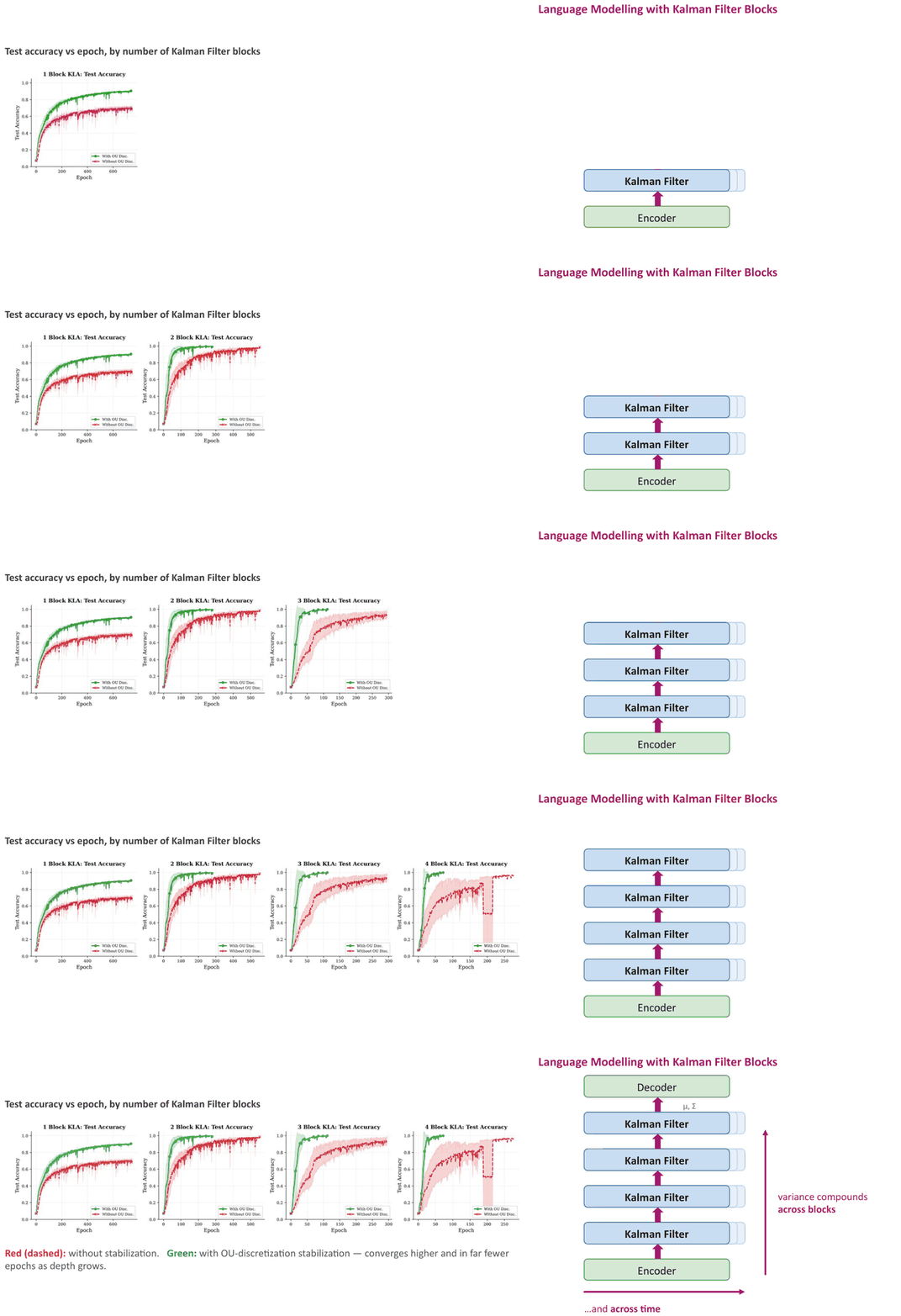
The fix turned out to be simple. It is not even a trick: deterministic SSMs such as S4 and Mamba already get their stability from discretising a well-behaved continuous-time ODE. We use the probabilistic counterpart of that idea, and set the prior dynamics of each filter to be a continuous-time Ornstein–Uhlenbeck (OU) process, which we then discretise. An OU process is mean-reverting: wherever the state wanders, it keeps getting pulled back towards a mean $m$, and its uncertainty settles to a fixed level instead of growing forever (Figure 4).

Discretising this prior keeps every filter inside the stable region by construction, for two reasons:
- The mean transition is contractive. Its eigenvalues are always less than one, so the mean cannot blow up, however deep the stack.
- The variance stays bounded. Each step’s prior variance becomes a convex combination of the current variance and the OU process’s long-run variance, so it can neither collapse to zero nor explode, and the divisions stay safe.
With the OU prior in place, training became much more stable: the green curves in Figure 3 converge higher, and in far fewer epochs, as the stack gets deeper. The exact discretisation formulas are in the paper
Kalman Filters Are Secretly Attention Maps
Just as you can unroll linear attention, Mamba or any other linear RNN into an attention matrix, you can unroll KLA. We unroll the posterior mean: the variance is trickier, because its Möbius recursion is non-linear.
Go back to the KLA recursion. In information form, the information mean $\eta_t = \lambda_t\,\mu_t$ (the posterior precision times the posterior mean) evolves as
\[\eta_t \;=\; {\color[RGB]{216,27,96}{f_t}}\,\eta_{t-1} \;+\; k_t\,{\color[RGB]{21,101,192}{\Lambda^{v}_t}}\,v_t, \qquad {\color[RGB]{216,27,96}{f_t}} \;=\; \frac{\bar{a}}{\bar{a}^2 + \bar{p}\,\lambda_{t-1}},\]where we fold the decay and the overwrite into a single term ${\color[RGB]{216,27,96}{f_t}}$. It acts as a history-dependent forget gate: unlike a Mamba gate, it depends on the filter’s precision $\lambda_{t-1}$, that is, on how certain the filter already is.
Dividing both sides by $\lambda_t$, and a little algebraic rearrangement (see the paper
The new ingredient is the precision ratio $\Lambda^{v}_t / \lambda_t$: the value precision of the current token, normalised by the filter’s total posterior precision (together with the key, it is the Kalman gain). It plays both roles at once. It is the input gate, setting how much of the new token gets written in; and it shrinks the forget gate $\bar{f}_t$, so the more of the new token is written in, the more of the old memory is overwritten. A confident filter (large $\lambda_t$) barely moves; a precise token (large $\Lambda^{v}_t$) moves it a lot.
Unrolling this over a sequence gives the posterior mean as $\mu = \mathbf{W}\,v$ (plus a term from the initial state), with
\[\mathbf{W} \;=\; \begin{pmatrix} k_1 {\color[RGB]{21,101,192}{\dfrac{\Lambda^{v}_1}{\lambda_1}}} & 0 & \cdots & 0 \\[10pt] {\color[RGB]{216,27,96}{\bar{f}_2}}\, k_1 {\color[RGB]{21,101,192}{\dfrac{\Lambda^{v}_1}{\lambda_1}}} & k_2 {\color[RGB]{21,101,192}{\dfrac{\Lambda^{v}_2}{\lambda_2}}} & \cdots & 0 \\[10pt] \vdots & \vdots & \ddots & \vdots \\[4pt] {\color[RGB]{216,27,96}{\prod_{s=2}^{T} \bar{f}_s}}\, k_1 {\color[RGB]{21,101,192}{\dfrac{\Lambda^{v}_1}{\lambda_1}}} & {\color[RGB]{216,27,96}{\prod_{s=3}^{T} \bar{f}_s}}\, k_2 {\color[RGB]{21,101,192}{\dfrac{\Lambda^{v}_2}{\lambda_2}}} & \cdots & k_T {\color[RGB]{21,101,192}{\dfrac{\Lambda^{v}_T}{\lambda_T}}} \end{pmatrix}.\]Like a causal attention matrix, $\mathbf{W}$ is lower-triangular: entry $(i, j)$ says how much the belief at step $i$ is shaped by the observation at step $j$. In other words, Kalman filters are secretly an attention mechanism.
Note that this is the attention matrix of the posterior mean alone, without the readout. Applying the readout adds the query, $y = q \odot \mu = \mathrm{diag}(q)\,\mathbf{W}\,v$, which in general gives a different pattern.
When we visualise these matrices for KLA models trained on the MAD-Lab tasks, the patterns are strikingly interpretable (Figure 5).

How Does It Perform?
Time to test each contribution empirically. Putting a Kalman filter on steroids, with a bit of maths and a bit of systems engineering, should buy us three things: speed over recurrent filters, expressivity from the non-linear recursion, and enough scale to pretrain LLMs. We check each in turn, take a look inside the filter at what its variance neurons learn, and finish with what happens when you drop a single KLA layer into a Transformer.
1. How Fast Is a Parallel Kalman Filter?
Let’s see how much of a performance improvement our parallel Kalman filter brings, compared with the sequential Kalman filter we discussed in Part 1, the kind that steers rockets but runs one step at a time. We profiled the wall-clock time of the forward and backward pass (that is, of training) on an A100 GPU, across sequence lengths, for four implementations of the same filter (Figure 6):
- The scan alone. Rewriting the recursion as a parallel scan, using PyTorch’s built-in associative scan (
torch._higher_order_ops.associative_scan), already buys roughly a 10× speed-up over the recurrent implementation in PyTorch at sequence lengths of 1–2k, with no custom code at all. - Fused kernels. Out of the box, each step of the scan reads its inputs from the GPU’s main memory (HBM) and writes its outputs back, so the computation is limited by memory traffic rather than arithmetic. Fusing the Möbius scan into a single Triton kernel cuts out most of those round-trips (see Making Deep Learning Go Brrrr From First Principles for why this matters), and buys another 3–6×.
- Staying in SRAM. Finally, like Mamba
, we avoid materialising the intermediate states in HBM at all: a CUDA kernel keeps them in the GPU’s small but fast on-chip SRAM. That brings a further speed-up of up to an order of magnitude at long context.
Put together, the fused CUDA filter is roughly 350× faster than the recurrent one at a sequence length of 2048, and it keeps running at 4096, where the recurrent and plain-PyTorch versions run out of memory. We will look at these implementation details more closely in Part 3.

2. Are the Explicit “Variance Neurons” Interpretable?
Unlike Mamba or linear attention, every channel of a KLA layer carries not just a mean but an explicit variance: a built-in “variance neuron” that says how uncertain the filter currently is. Do these neurons learn anything interpretable?
To find out, we visualised the posterior variance of a KLA model trained on the MAD-Lab Selective Copy task, where the model has to remember a handful of marked tokens scattered among distractors and blanks, and reproduce them when it sees a COPY signal (Figure 7).

Two patterns stand out. First, the variance falls steadily over the sequence: as evidence accumulates, the filter becomes more certain about its state. Second, it spikes sharply at exactly the positions that matter, the tokens the model will later have to copy. A spike in variance means a large Kalman gain, so these are the moments where the filter “opens up” and lets the new token overwrite its belief, while distractors and blanks barely move it. In other words, the variance neurons act as an interpretable, uncertainty-driven gate: selection falls out of uncertainty propagation rather than from a hand-designed gate.
We use these plots as a window into the filter’s internal dynamics, not as a claim that the variances are calibrated uncertainty estimates. Making them calibrated is an interesting direction of its own.
3. What Does Non-Linearity Buy? State Tracking
What does the non-linear, Möbius-style recursion actually buy us? One answer is state tracking: keeping track of how the state of a world changes as a sequence of actions is applied to it. This is a well-known weakness of linear recurrences such as Mamba, and of Transformers too
To test this, we used the $A_5$ benchmark from the same paper

And that is exactly what we see. Mamba and Transformers need more and more blocks as the task gets harder, that is, as the prediction horizon grows, climbing to four. A classical RNN gets away with a single block, thanks to its non-linear recurrence, but it cannot be trained in parallel. KLA sits in between: its non-linearity, which comes from the precision recursion, lets it solve the task with two blocks at every horizon we tried, while still training in parallel.
So we finally have a primitive that is non-linear, yet parallelisable.
4. Does It Scale to Language Modelling?
Finally, does any of this survive contact with real language? We trained KLA language models of up to 180 M parameters (on 10.9 B tokens at the 180 M scale), both on their own and as hybrids, and evaluated them zero-shot on eight standard commonsense-reasoning benchmarks (Table 3).

Even with the simplest assumptions we made, time-invariant dynamics and very little tuning, standalone KLA already has the best average of all the standalone models at both scales (37.68 at 45 M and 42.78 at 180 M, against 37.08 and 42.30 for Mamba). It seems particularly strong on the reasoning-heavy benchmarks: it is best or tied-best on BoolQ at both scales, best on HellaSwag at 180 M, and within a fraction of a point of the best on WinoGrande. Most probably, that is the state-tracking capacity and the extra expressiveness of the non-linear recursion paying off. There is still room for improvement on recall: LAMBADA, the benchmark that leans most on retrieving a specific earlier word, lags behind. That is the known trade-off for any model with a fixed-size state, and something we are still working on.
5. One KLA Layer in a Transformer
To isolate the effect of the layer itself, we took a 12-layer GPT and replaced only its last attention layer with a recurrent one, so that eleven layers stay softmax attention and the twelfth is Mamba, Gated DeltaNet or KLA. Which works best (Figure 9)?

Every hybrid helps a little, but KLA helps the most: at 180 M, swapping in one KLA layer lifts the average from 42.20 to 44.95, against 43.28 for Gated DeltaNet and 42.25 for Mamba. Even as a single layer, KLA seems to complement a Transformer very well.
That’s the end-to-end story. Möbius composition turns a recurrence into a parallel scan, OU bounding keeps deep stacks stable, and end-to-end learning turns a hand-tuned filter into a general primitive. What you get out the other side is a mixer that is cheap like an SSM, expressive enough to track state in half the depth, and that hands you a calibrated variance at every token — which, going back to where we started, is the quantity a model needs when it has to decide whether to act rather than just what to say.
The next post (Part 3) goes under the hood with more implementation details. In the meantime, the paper and the project page have the full details.
Additional details: state expansion
Our first KLA filter used a plain diagonal vector state, with one mean and one variance per channel. On the MAD-Lab benchmark it performed poorly. Following Mamba, we added state expansion (the dimension called d_state in Mamba codebases): each channel's scalar state is expanded into a larger state of size d_state, and the overall state dimension grows accordingly.
For the mean, state expansion is straightforward to reason about, just as for any other linear RNN with a matrix-structured state. The covariance is subtler: what it should look like depends on the modelling assumptions you make in the underlying graphical model. Two readings are natural:
- Independent filters. Treat each expanded state dimension as a separate filter of its own. The filters are independent, even though they all see similar observations (values). Under this reading, the covariance stays exactly diagonal.
- One mixed filter. Treat each value as generated from the whole expanded state, so the observation model mixes the expanded state dimensions. An exact filter would then need a full covariance over the expanded state, and our diagonal update equations should be read as a diagonal approximation to it.
See the appendix of the camera-ready paper
Image credits: flying superhero icon designed by Freepik.