Kalman Linear Attention 1: A Beginner's Guide to Kalman Filters

An intuitive introduction to Kalman filters - from state observers to predict-update recursions - and why they matter for modern sequence models

Part 1 of a series connecting classical Bayesian filters to modern linear-attention sequence models.

What if I told you that the same recursive algorithm that steered Apollo 11 to the moon, that helps neuroscientists decode signals from the visual cortex, and that runs inside every smartphone GPS — is, with a one-line reparameterisation, a linear-attention layer for modern sequence models?

That algorithm is the Kalman filter: sixty-five years old, trusted everywhere engineers need to infer the hidden state of a noisy world from partial observations of it. This three-part series shows how it becomes Kalman Linear Attention (KLA) — a drop-in replacement for softmax attention with linear-time inference, parallel training, and calibrated uncertainty for free.

This first post is the filter itself: the minimum working mental model — no prerequisites beyond basic linear algebra and probability. Already fluent in predict-update? Skip ahead to Part 2, where the same recursion turns into an attention layer.

The journey. §1 builds intuition · §2 sets up the stochastic SSM in which filtering / state estimation is performed · §3 states the problem the KF solves · §4 when and why is it the “best” of all estimators? :) · §5 sketches the derivation of the recursion · §6 watches one work on a James Bond 🕶️ scenario · §7 points to further references.

---

1. What Is a Kalman Filter?

A Kalman filter is a state observer / estimator - a recursive estimator that infers the latent state (the hidden quantities the world keeps from you) of a (stochastic) black-box physical system from a stream of noisy, partial observations of it. The eye in Figure 1 is more than a metaphor: mathematically, a state observer / estimator is a piece of code that consumes observations $y_{1:t}$ and produces an estimate $\hat x_t$ of “what the world looks like, given what I’ve seen so far”. The Kalman filter is one specific - and very famous - observer: the optimal linear one for a particular class of models.

Figure 1. The unknown system + observer frame the rest of the post lives in. The top box is the world - possibly non-linear, possibly stochastic, with hidden state $x_t$. The bottom box is the observer (the eye is its job: looking at the world through the only window it has, $y_t$). The Kalman filter is the specific observer we'll build.

The KF’s inference equations are derived from a particular linear choice for the system functions $f$ and $g$ above, and a Gaussian white-noise assumption (sometimes weaker - see below). We’ll lay out that model in §2 next.

---

2. Linear Noisy State-Space Models

We have an unknown system and want to infer its underlying state in real time from a stream of observations. To get anywhere we have to commit to a simplified generative model of how the world produces those observations - with the simplifications chosen so that

1. inference is tractable in real time for the use case (constant compute and memory per step), and
2. the modelling errors and uncertainties introduced by those simplifications are absorbed into explicit noise terms - so the filter always knows what it doesn’t know.

Concretely, the Kalman filter’s simplification is exactly the one previewed at the end of §1: take the transition and observation functions $f, g$ to be linear, and let the noise terms $\omega_t, \gamma_t$ absorb every unmodelled effect. Spelled out, that gives the following linear state-space generative model.

1. Linear dynamics. The latent state evolves linearly in time: \[x_{t+1} \;=\; A_t\, x_t \;+\; B_t\, u_t \tag{2.1}\] where $u_t$ is an optional control input. In unactuated settings - the most relevant for language modelling used in KLAKLA = Kalman Linear Attention, the technique built in Part 2 - a Kalman recursion wrapped in a deep encoder with all four matrices learned. - $B_t u_t$ is absent. 2. Process noise ($\omega_t$) absorbs everything else (mild non-linearities, model errors, external disturbances): \[x_{t+1} \;=\; A_t\, x_t \;+\; B_t\, u_t \;+\; \omega_t \tag{2.2}\] 3. Linear observation model. What you see is a linear function of the state: \[y_t \;=\; C_t\, x_t \tag{2.3}\] 4. Observation noise ($\gamma_t$). Sensors are noisy - same trick: \[y_t \;=\; C_t\, x_t \;+\; \gamma_t \tag{2.4}\] 5. White noise. $\omega_t$ and $\gamma_t$ are zero-mean, uncorrelated across time, with finite (constant) covariance: \[\Sigma^{\mathrm{proc}} = \mathbb{E}\!\left[\omega_t \omega_t^{\top}\right], \quad \Sigma^{\mathrm{obs}} = \mathbb{E}\!\left[\gamma_t \gamma_t^{\top}\right] \tag{2.5}\]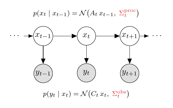

Figure 2. The five assumptions drawn as a graphical model. Latents $x_t$ form a hidden chain (top); each emits a noisy observation $y_t$ (bottom). Shown is the Gaussian special case - the typical textbook form. Under just white noise (per the callout below), the same equations describe only the first two moments of the conditionals.

🟦 On the Myth of Gaussianity Being Necessary. Notice that Gaussianity was nowhere on the assumption list above - that absence is deliberate, not an oversight. The PGM in Figure 2 draws the Gaussian special case only because it makes the textbook Bayesian derivation closed-form; Kalman’s 1960 derivation itself never requires it. Two precise takeaways:

1. Gaussianity isn’t needed to write down or run the Kalman recursion. Kalman’s derivation leaves $p(x_t \mid x_{t-1})$ and $p(y_t \mid x_t)$ as arbitrary, unspecified distributions and characterises them only through their first two conditional moments - the conditional expectations $\mathbb{E}[x_t \mid x_{t-1}] = A_t x_{t-1}$, $\mathbb{E}[y_t \mid x_t] = C_t x_t$ and the conditional covariances $\mathrm{Cov}[x_t \mid x_{t-1}] = \Sigma^{\mathrm{proc}}_t$, $\mathrm{Cov}[y_t \mid x_t] = \Sigma^{\mathrm{obs}}_t$ - with the densities $p(\,\cdot \mid \cdot\,)$ themselves never committed to a parametric form. The closed-form recursive estimator is derived from these alone, via optimisation - no Gaussian density ever invoked.
2. Gaussianity sharpens the optimality claim - it doesn’t unlock the algorithm. Without it, the recursion is the best linear-MSE estimator (no linear estimator beats it; nonlinear ones in principle could). With Gaussianity - or just symmetry+unimodality of the posterior - the same equations deliver the true conditional mean $\mathbb{E}[x_t \mid y_{1:t}]$, which is the best estimator among all reasonable estimators under MSE. Same equations, strictly stronger guarantee. Kalman 1960 lays out the full hierarchy of optimality theorems spanning these (loss, distribution) regimes; we work through them in §4.

2.1. Is the Linear Assumption Too Restrictive?

Looking at that list it’s tempting to say “linear dynamics + linear observations? My problem isn’t like that at all.” In practice the filter is surprisingly robust for two reasons.

1. The noise term is a load-bearing fudge factor. Anything you didn’t model - slow drifts, sensor biases, mild non-linearities - gets absorbed into $\omega_t$ and $\gamma_t$. The covariances $\Sigma^{\mathrm{proc}}$ and $\Sigma^{\mathrm{obs}}$ are tuning knobs that tell the filter how much to trust its dynamics versus its sensors.

2. A wrong-but-good-enough model with reasonable noise estimates can still produce excellent state estimates - online, recursively, in constant memory. The filter doesn’t need to be the truth; it needs to be useful.

If you want richer expressivity - non-linear latent dynamics, learned features, hierarchical structure - replace the handcrafted matrices with neural networks: process incoming sensory signals through a neural feature extractor and do filtering in a non-linear latent space. We’ll explore that path in Part 2: from the linear KF to Kalman Linear Attention (KLA).

---

3. Toward the KF Update Equations: State Estimation via Optimization (and its Inference Dual)

Earlier we framed the KF as a state observer - a black-box consumer of $y_{1:t}$ that emits a state estimate $\hat x_t$. But how does that estimation actually work? The KF update equations can be seen as solutions to one well-posed problem with two equivalent statements: either (i) solving an optimisation objective with a specific loss $L$, or (ii) doing probabilistic inference on a specific directed graphical model - the Linear Gaussian State Space Model (LGSSM) PGM drawn earlier (Figure 2, the Five Assumptions graphical model). We write both statements here. §5 walks through how the recursion is derived from either one (optional reading), and §5.1 (The Predict–Update Cycle) shows what the recursion does at each step.

Statement A - optimisation. Given $y_{1:t}$, find the estimator that minimises an expected loss

\[\hat x_t \;=\; \arg\min_{\hat{x}}\; \mathbb{E}\!\left[\,L(x_t - \hat{x}) \,\big|\, y_{1:t}\,\right]. \tag{3.1}\]

Statement B - inference (the dual). Given the same $y_{1:t}$, compute the posterior over the latent state

\[p(x_t \,\big|\, y_{1:t}), \tag{3.2}\]

and report a summary of it - by default, its mean.

🟦 (A) and (B) Coincide on the LGSSM but importantly not the only case where this can coincide. Kalman 1960 pins down the precise conditions under which the optimisation statement (3.1) and the inference statement (3.2) yield the same answer - illustrated in Figure 3, with the broader duality map detailed in the toggle below (optional).

🟦 The Take-Away for the Rest of This Post. The (A) ↔ (B) duality isn’t a hand-wavy observation - Kalman 1960 establishes it rigorously via a small hierarchy of optimality theorems (Thm 1, 1-a, 2 - laid out in §4) that hold across surprisingly general regimes of loss and distribution. A practical consequence: because the two sides of the duality provably coincide, the same Kalman recursion can be re-derived from the native toolkit of whichever field one is most fluent in - optimisation (orthogonal projection in $L^2$$L^2$ is the Hilbert space of square-integrable random variables - random variables $X$ with $\mathbb{E}[X^2] < \infty$ - equipped with inner product $\langle X, Y \rangle = \mathbb{E}[XY]$ and norm $\|X\| = \sqrt{\mathbb{E}[X^2]}$. The norm-squared is precisely the MSE, so minimising MSE = minimising squared distance in $L^2$, and the best linear estimator is the orthogonal projection of $x_t$ onto the linear span of past observations $\{y_1, \ldots, y_t\} \subset L^2$. Not to be confused with $\ell_2$ (lowercase $\ell$), which in ML usually refers to finite-dimensional weight regularisation / squared loss.), probabilistic inference / graphical models (message passing on the LGSSM PGM similar to HMMs), information geometry (KL projection onto a Gaussian manifold), and so on. In every case the target object is the same: $\mathbb{E}[x_t \mid y_{1:t}]$.

(Optional / Advanced) Mapping the (A. Optimization) ↔ (B.Inference) duality region - where does the Kalman recursion live? →

The precise duality conditions. Kalman 1960 lays this out in two theorems: under MSE, no distributional assumption on the posterior is needed (Thm 1-a); under broader losses, symmetry+unimodality of the posterior suffices (Thm 1). Spelling out the equality:

\[\underbrace{\arg\min_{\hat{x}}\;\mathbb{E}\!\left[\,L(x_t-\hat{x}) \,\big|\, y_{1:t}\,\right]}_{\text{optimum of (A)}}\;\;=\;\;\underbrace{\mathbb{E}\!\left[\,x_t \,\big|\, y_{1:t}\,\right]}_{\text{mean of (B)}} \tag{3.3}\]

holds in two cases (Figure 3 below):

• Squared-loss case (Thm 1-a). For $L(\varepsilon)=\varepsilon^{2}$ (MSE), the equality holds for any distribution - no symmetry or unimodality needed. $\mathbb{E}[x_t \mid y_{1:t}]$ is simply the $L^{2}$-projection of $x_t$ onto the observations.
• General-loss case (Thm 1). For any “reasonable” loss $L$ - symmetric, non-decreasing in $\lvert\varepsilon\rvert$, e.g., $\lvert\varepsilon\rvert$, $\varepsilon^{4}$, $1-e^{-\varepsilon^{2}}$ - the equality holds provided the posterior is symmetric and unimodal. Gaussian is the canonical instance (symmetric and unimodal by construction), and the LGSSM gives us this for free.

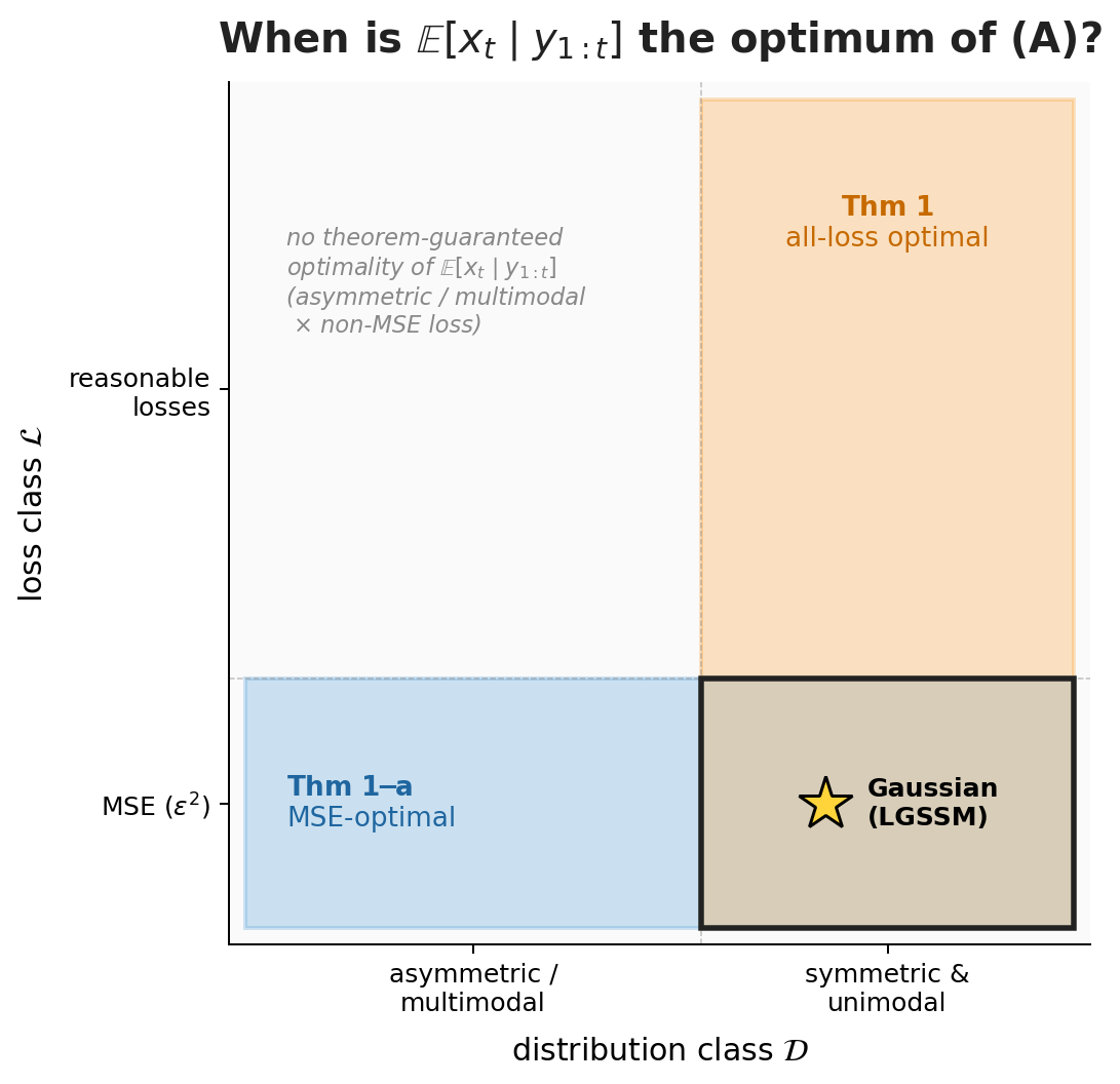
_{Figure 3. Each Kalman 1960 theorem picks out a rectangle in the $(\mathcal{L}, \mathcal{D})$ plane on which $\mathbb{E}[x_t \mid y_{1:t}]$ is the optimum of (A).
Thm 1-a = horizontal strip (MSE $\times$ any distribution); Thm 1 = vertical strip (any reasonable loss $\times$ sym+uni).
They cross at MSE $\times$ sym+uni - Thm 1's stronger all-loss claim dominates there.
Gaussian (and hence the LGSSM) lives in the intersection.}

Where the Kalman recursion sits on this map. The recursion we derive in §5 is constrained to the LGSSM corner: linear dynamics $+$ linear observations $+$ MSE loss $+$ Gaussian (or just sym+uni) noise. That corner sits inside the intersection cell of the strips diagram - both theorems apply, and the conditional mean is optimal under any reasonable loss. The wider map matters because it tells us the duality (A) ↔ (B) holds far beyond the LGSSM corner - but practical, recursive, closed-form algorithms only exist inside it. KLA in Part 2 will be a controlled departure from the corner, via data-dependent dynamics.

Why the dual view is useful. Holding (A) and (B) as two faces of the same problem matters chiefly when you want to derive the recursion from scratch (as sketched in §5) - different techniques (loss-minimization, posterior-update, orthogonal projection) start from different sides of the duality and land on the same equations. For just using the recursion, the intuition alone is enough: state estimation can be cast either way, and the two views coincide on the LGSSM.

---

4. Best Linear Estimator under MSE Loss

Suppose we restrict ourselves to linear estimators - i.e. estimators that are a linear function of past observations $(y_{1:t})$,

\[\hat x_t \;=\; \sum_{s \,\leq\, t} \alpha_s\, y_s, \tag{4.1}\]

where each $\alpha_s$ is a real-valued (matrix-valued in general) coefficient applied to past observation $y_s$ - one matrix per time index. The $\alpha_s$ aren’t fixed in advance; they are picked by the estimator / optimisation algorithm itself, as whatever values minimise the optimisation objective in eq (3.1) - equivalently, whatever values realise the inference summary in eq (3.2). Theorem 2 below then characterises that optimal pick - it turns out to coincide with the orthogonal-projection coefficients (see the toggle).

Kalman’s Theorem 2 says that, within this class of linear estimators, the optimum under squared (MSE) loss is achieved by the Kalman recursion - and, crucially, no distributional assumption on the noise processes $\omega_t, \gamma_t$ is needed for this to hold. Just second moments. No Gaussianity, no symmetry, no unimodality. The Kalman filter is therefore the gold-standard linear-MSE estimator for any linear state-space model: nonlinear estimators (particle filters, nonlinear smoothers) can in principle do better, but no linear one can.

(Optional) Why this matters operationally - orthogonal projection, recursivity, and the Apollo connection →

The geometric form. Theorem 2 says more than “an optimum exists” - it gives that optimum a concrete geometric form. The optimal linear estimate \hat x_t = \sum_{s \le t} \alpha_s\, y_s from eq (4.1) is the orthogonal projection \Pi_{\mathcal{H}_t}(x_t) of the latent state x_t onto the closed linear span \mathcal{H}_t of past observations y_{1:t}. The coefficients \alpha_s are then defined by the orthogonality condition - the residual must be uncorrelated with every past observation:

\mathbb{E}\!\left[(x_t - \hat x_t)\, y_s^{\top}\right] \;=\; 0 \qquad \text{for all } s \leq t. \qquad\qquad (4.2)

Solving this system gives the explicit form of each \alpha_s.

The geometry the projection exposes - each new observation contributes only its unpredictable, orthogonal component (the innovation: the part of y_t not linearly predictable from $y_{1:t-1}$); whatever was already predictable from the past adds nothing new - is precisely what lets the optimum of eq (3.1) (equivalently, the conditional-mean summary of eq (3.2)) be computed recursively, one observation at a time, in constant memory, rather than as a batch re-solve over the full history. Conditional expectations in general do not compose this way - the projection structure is doing real work.

That compute-friendly recursive form is what made the Kalman filter the workhorse of real-time navigation in the Apollo program (where on-board memory was measured in kilobytes), and the default tool for robotics, GPS, and control ever since. The same recursion also returns a covariance P_t tracking the second-moment uncertainty in the estimate.

The orthogonal-projection geometry itself is unpacked further in §5 - and there we will additionally derive the very same predict–update recursion using a different tool: Bayesian inference on the LGSSM viewed as a probabilistic graphical model (HMM-style message passing). For an ML audience that has already seen HMMs / belief propagation, that second route is often the more familiar one - and it lands on exactly the same equations.

🟦 Relevance to modern linear RNN / SSM literature. Linear RNNs and linear SSMs are - by construction - linear functions of their input history. Thm 2 says we cannot theoretically do better than the Kalman recursion in an MSE sense within that class. The Kalman filter is the gold-standard linear MSE estimator for any linear state-space model. Beating it requires breaking linearity-in-input - via nonlinear smoothers, particle filters, attention, or data-dependent dynamics (selective SSMs like Mamba and KLA - exactly Part 2’s story).

Under Gaussianity: even stronger. Kalman’s own commentary on Thm 2 notes that Gaussianity broadens the result further. If the underlying process is in fact Gaussian (more generally: symmetric+unimodal posteriors - see the case-split inside the toggle in §3), Thm 1 promotes the Kalman estimator from “best linear under MSE” to “best estimator overall, under every reasonable loss.” This isn’t irrelevant for what follows - there are KLA / SSM applications where the data are at least approximately Gaussian, and you get the stronger all-loss guarantee for free. And when Gaussianity doesn’t hold, Thm 2 alone - best linear MSE estimator - is already enough to make the Kalman recursion a very strong choice.

---

5. Explaination and Derivation of the Update Equations

As a headsup only understanding what the update equations is a necessary primer for KLA in part 2, the full on derivations are not required and are discussed only for completeness.

As discussed in §3, the inference ↔ optimisation duality on the LGSSM means the same Kalman recursion can be derived from several different toolboxes - each starting from a different side of the duality and landing on the same equations. We’ll call these points of view (POVs).

Regardless of which POV one takes, every derivation of the KF threads through two canonical steps:

1. Prediction (a.k.a. time update) - given past observations $y_{1:t-1}$, what is my best guess for the system state at the next time step $t$, before seeing the new observation $y_t$?
2. Update (a.k.a. observation update) - now fold the fresh observation $y_t$ into that prediction, to get the best guess for the system state at time $t$ given all observations $y_{1:t}$ so far.

The toggle below sketches two such POVs - one via optimisation, one via probabilistic inference on the LGSSM PGM - showing how each threads through these two steps and lands on the same recursion. The full derivations are beyond the scope of this primer and may be covered in separate posts; open the toggle only if you’d like intuition for the different tools one can use to derive the KF (and adapt them to your own SSM variants beyond the simple linear-Markovian case - switching models, hierarchical models, etc.). The Predict–Update cycle in §5.1 below is what you actually need to follow Part 2.

(Optional) Sketch of the two KF derivations - via the inference / optimisation duality (§3) →

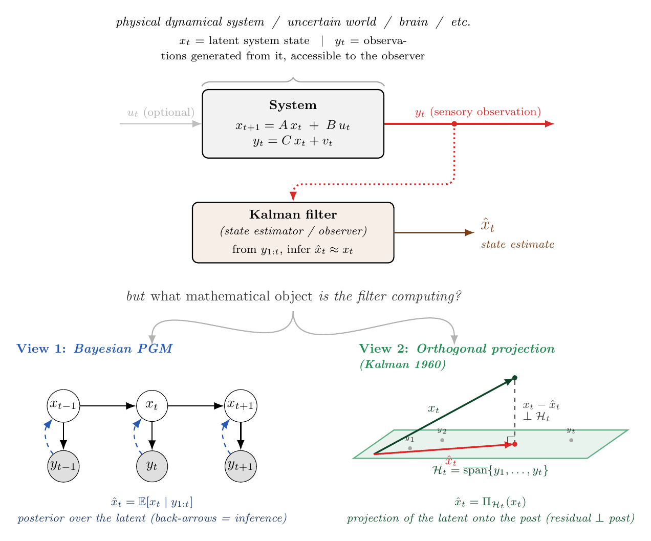
Figure 4. Two POVs, identical recursion. Top: a recap of the system + observer frame. Bottom-left (POV 1): Bayesian posterior inference on the graphical model, with dashed back-arrows highlighting the direction of information flow during the update step. Bottom-right (POV 2): Kalman’s original 1960 derivation - the optimal linear estimate is the orthogonal projection of $x_t$ onto the subspace $\mathcal H_t$ spanned by past observations, with the residual error perpendicular to that subspace.

Recall from §3 that we established the (A) optimisation ↔ (B) inference duality: the optimal Kalman estimate can be defined either as the minimiser of an expected squared loss (eq 3.1) or as the conditional-mean summary of a posterior (eq 3.2). The two points of view below correspond to attacking the recursion through one side of that duality or the other - POV 1 from the inference side (B), POV 2 from the optimisation side (A) using the orthogonal-projection tool that Thm 2 (§4) handed us. They land on the same equations because, on the LGSSM, the two sides coincide; which one feels more natural depends on your background.

POV 1 — Probabilistic inference on the LGSSM PGM

(the (B) / inference side of the §3 duality)

This is the standard-toolbox route, familiar to anyone who’s seen the HMM forward pass for discrete state-spaces - the linear-Gaussian case is its continuous-state analogue. The goal at each step is to compute the filtering posterior

\[p(x_t \,\big|\, y_{1:t}) \tag{5.1}\]

on the LGSSM viewed as a graphical model (latents $x_0 \to x_1 \to \cdots$ generate observations $y_t$; the filter inverts the generative arrow to infer the latent - forward solid arrows = generative, dashed back-arrows = inference). By Bayes’ rule, the posterior factorises into a likelihood times a prior, normalised by the marginal evidence:

Update step — Bayes' Rule (eq 5.2) p(x_t \mid y_{1:t}) \;=\; \frac{\overbrace{p(y_t \mid x_t)}^{\text{likelihood}} \;\; \overbrace{p(x_t \mid y_{1:t-1})}^{\text{prior}}}{\underbrace{p(y_t \mid y_{1:t-1})}_{\text{normaliser}}}

Under the LGSSM, all three factors are Gaussian, so the product (and quotient with the normaliser) stays Gaussian and this update step admits a closed-form solution.

The prior $p(x_t \mid y_{1:t-1})$ in eq (5.2) is not free - it has to be predicted from the previous posterior by marginalising over $x_{t-1}$. The standard tool is the Chapman–Kolmogorov equation (the law of total probability applied to a Markov chain):

Prediction step — Chapman–Kolmogorov (eq 5.3) \underbrace{p(x_t \mid y_{1:t-1})}_{\text{prior at } t} \;=\; \int \underbrace{p(x_t \mid x_{t-1})}_{\text{transition model}} \;\; \underbrace{p(x_{t-1} \mid y_{1:t-1})}_{\text{previous posterior}} \, dx_{t-1}

Again, both factors inside the integral are Gaussian under the LGSSM, so this prediction step also collapses to a closed-form Gaussian.

Together, eq (5.3) (Chapman–Kolmogorov prediction) and eq (5.2) (Bayes update) give the Predict–Update cycle that §5.1 below unpacks concretely. The derivation reuses standard machinery from any inference / PGM course - message passing on the chain, conjugate Gaussian priors, a few Gaussian identities looked up in any textbook. Mechanical and cheap. The catch: it leans on the Gaussianity assumption; outside that, the recursion no longer closes in finite-dimensional sufficient statistics, and nonlinear / non-Gaussian extensions (EKF, UKF, particle filters) become necessary.

POV 2 — Orthogonal projection in Hilbert space

(Kalman 1960; the (A) / optimisation side of the §3 duality)

If you haven’t seen $L^2$ / Hilbert spaces before, POV 1 above already gives the same recursion via different machinery - feel free to skip POV 2 on first reading. The rigorous derivation is in Kalman’s original 1960 paper; what follows is the geometric intuition.

Setup. Treat every random vector as a point in the Hilbert space $L^2$ with inner product $\langle X, Y \rangle = \mathbb{E}[XY]$. Let $\mathcal H_t$ be the closed linear span of past observations $y_1, \ldots, y_t$. Kalman defines the estimate $\hat x_t$ as the orthogonal projection of the true latent onto $\mathcal H_t$:

\[\hat x_t \;=\; \Pi_{\mathcal H_t}(x_t). \tag{5.4}\]

Geometrically: drop a perpendicular from the point $x_t$ onto the subspace spanned by all observations seen so far. The residual $x_t - \hat x_t$ is then perpendicular to every $y_s$, $s \le t$ — that’s the orthogonality principle $\mathbb{E}[(x_t - \hat x_t)\, y_s^\top] = 0$.

Why this leads to a recursion - Gram–Schmidt on the fly. Naively, projecting onto a $t$-dimensional subspace would require inverting a $t \times t$ Gram matrix - quadratic memory, cubic compute, no good. Kalman’s trick: orthogonalise the observations one at a time as they arrive, so each step only has to handle one new direction.

Walk through it concretely. At $t = 1$, $\mathcal H_1$ is a single direction $y_1$, and $\hat x_1$ is just the projection of $x_1$ onto that line. At $t = 2$, a new observation $y_2$ arrives. Decompose it orthogonally into the part already lying in $\mathcal H_1$ plus a new perpendicular component:

y_2 \;=\; \underbrace{\hat y_{2 \mid 1}}_{\text{predictable from } y_1} \;+\; \underbrace{\tilde y_2}_{\text{innovation } \perp \mathcal H_1}

where $\hat y_{2 \mid 1} = \mathbb{E}[y_2 \mid y_1] \in \mathcal H_1$ is the part of $y_2$ that was already in the old subspace, and $\tilde y_2 = y_2 - \hat y_{2 \mid 1}$ is the innovation — what’s genuinely new, perpendicular to $\mathcal H_1$. Crucially, ${y_1, \tilde y_2}$ is now an orthogonal basis for $\mathcal H_2$, and projecting onto an orthogonal basis is trivial: the projection of $x_2$ is just the sum of projections onto each basis vector — projection onto the old direction $y_1$ plus projection onto the new innovation direction $\tilde y_2$.

The same structure holds at every step. The projection of $x_t$ onto $\mathcal H_t$ decomposes as the projection onto the old subspace $\mathcal H_{t-1}$ (the prior) plus a correction along the single new innovation direction:

Recursive update — prior + innovation correction (eq 5.5) \hat x_t \;=\; \underbrace{\hat x_{t \mid t-1}}_{\text{prior}} \;+\; \underbrace{K_t \, \tilde y_t}_{\text{correction along innovation}}

Here $\hat x_{t \mid t-1} = \Pi_{\mathcal H_{t-1}}(x_t)$ is the projection onto past observations — what we’d estimate from history alone, exactly POV 1’s prior $\mathbb{E}[x_t \mid y_{1:t-1}]$. The Kalman gain $K_t$ is the coefficient of the projection onto the new innovation direction $\tilde y_t$ — fixed by demanding the residual be perpendicular to $\tilde y_t$ (one-direction projection, cheap). A few lines of linear algebra turn $\hat x_{t \mid t-1}$ and $K_t$ into the closed-form Kalman recursion (see Kalman 1960 for the rigorous derivation).

The geometric pay-off: every new observation contributes only the part of itself that’s orthogonal to everything seen before. That’s what lets the recursion run in constant memory per step rather than re-solving over the full history.

Optimality. Theorem 2 of Kalman’s paper says this projection is the optimal estimator under squared loss within the linearity restriction, without any Gaussianity assumption; Theorem 1 (after Sherman 1958) lifts that to every reasonable loss whenever the posterior is symmetric and unimodal. This is the picture a signal-processing or statistics reader has, and it is what Kalman actually wrote in 1960, long before “Bayes nets” were standard. (See the case-split bridge in §3 above for the precise theorem statements.)

There are plenty of other routes too - exponential-family conjugacy, variational free energy, recursive least squares, you name it. Pick the comfort zone closest to your background; the recursion at the end is the same. (For the precise sense in which the result is “optimal” - and why our LGSSM gets a stronger guarantee than just MSE - see the case-split (Thm 1 vs Thm 1-a) in §3 above.)

For jointly Gaussian variables the two POVs are formally identical

• conditional expectation = orthogonal projection. Pick the picture that fits your audience and the rest of the math is bookkeeping.

What you actually need to carry into Part 2. You will not rederive any of this. What matters is: at every step the KF emits a pair $(\mu_t, P_t)$ - posterior mean and covariance - and these obey a linear recursion in those quantities, equivalently in the natural parameters $(\Lambda_t, \eta_t)$. Some linear algebra turns the predict–update cycle into the closed-form Kalman equations; which derivation got you there (orthogonal projection, Bayes’ rule, exponential-family conjugacy) is a matter of taste. Part 2 holds the recursion structure fixed and reparameterises it for parallel computation - it does not rederive it.

5.1. The Predict-Update Cycle

To make what the filter does at each step concrete, here is what happens to its belief between two observations:

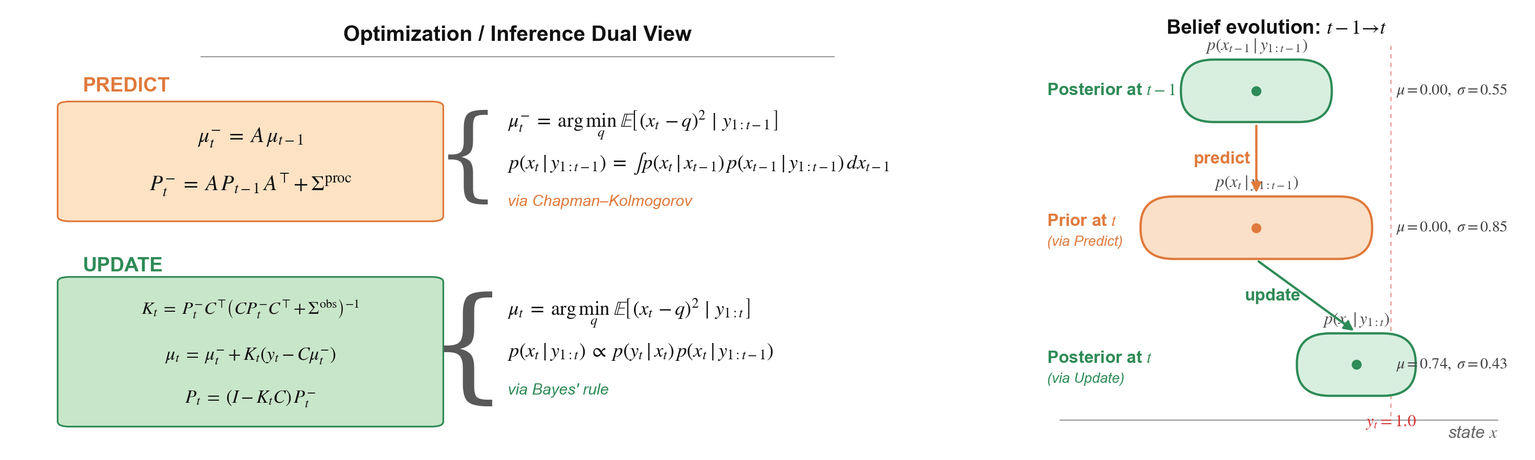
Figure 5. The predict–update cycle, two views.

Left: the predict step can be cast as either solving an optimisation problem (argmin of expected squared error from past observations) or doing inference. For the NLP / HMM reader, that inference is just the marginalisation substep of the forward algorithm - known in continuous state-spaces as the Chapman–Kolmogorov equation. The update step is similarly either an optimisation (argmin after folding in the latest $y_t$) or inference - the conditioning substep of the forward algorithm, i.e. Bayes’ rule applied to $y_t$. On the LGSSM both views collapse to the same closed-form recursion shown below each.

Right: visual intuition on how the belief evolves on a 1D state axis. The dot is the mean (first moment); the shaded region around it is the variance (second moment) — only these two moments are committed, no Gaussianity required (matching Thm 2 of §4). posterior at $\textcolor{#2E7D32}{t-1}$ → predict widens it to the prior at $\textcolor{#C66A00}{t}$ (variance grows by additive process noise $Q$) → update folds in the observation $\textcolor{#D32F2F}{y_t}$, giving a tighter posterior at $\textcolor{#2E7D32}{t}$. Predict always widens uncertainty; update always tightens it — or, in the worst case (missing observation $\equiv$ infinite observation variance / zero precision), leaves it equal. Update never makes things worse.*

For reference - the closed-form LGSSM recursion shown inside Figure 5, written out for copy-paste convenience.

Predict step - propagate the previous posterior through the dynamics:

\[\mu_t^- \;=\; A\, \mu_{t-1}, \qquad P_t^- \;=\; A\, P_{t-1}\, A^{\!\top} + \Sigma^{\mathrm{proc}} \tag{5.3}\]

Update step - fold in the new observation $y_t$ via the Kalman gain $K_t$:

\[K_t \;=\; P_t^-\, C^{\!\top} \bigl(C\, P_t^-\, C^{\!\top} + \Sigma^{\mathrm{obs}}\bigr)^{-1} \tag{5.4}\] \[\mu_t \;=\; \mu_t^- + K_t\,(y_t - C\, \mu_t^-), \qquad P_t \;=\; (I - K_t C)\, P_t^- \tag{5.5}\]

---

6. A Classical Kalman Filter in Action

Enough abstraction. Let’s see one work.

🎬 The setup. James Bond is on vacation, having a private call in a closed 1-D corridor. His security agency wants to track his movements for safety without compromising privacy - they only have an inexpensive, noisy position sensor on his phone. The agency uses a Kalman filter to fuse the sequence of sparse, noisy sensor readings and estimate / predict in real time Bond’s position and velocity.

Figure 6. The full pipeline in motion. Watch the orange ghost overshoot during predict steps, the green posterior snap back at every ping, and the velocity panel quietly track the truth even though it never receives a single direct observation.

6.1. What to Watch in the Animation

A quick tour of the four panels, top to bottom:

Top - graphical model + predict/update. Kalman filtering viewed as posterior inference in an SSM. The predict step rolls the latent $x$ forward through the causal dynamics $(A, \Sigma^{\mathrm{proc}})$ to give the prior $p(x_t \mid y_{1:t-1})$; the update step performs a Bayesian inversion - the green dashed back-arrow $y_t \to x_t$ in the PGM - to fold in the new noisy observation and give the posterior $p(x_t \mid y_{1:t})$. When no ping arrives at a step, we simply carry the prior forward.

Second row - position over time. True position $p_t$ in blue; noisy position sensor data ($y_t$) as red dots; filter mean $\hat{\mu}_p$ in orange, with the $\pm 2\sigma$ uncertainty band shaded around it.

Third row - velocity over time. Same colour scheme for the latent velocity, except there are no red dots (🔴) - no velocity sensor exists. The filter must infer velocity purely from the pattern of incoming position sensor data.

Bottom - 1-D corridor (spatial view). Bond (solid blue 🧍) paces the corridor in real time; the dashed ghost is the filter’s belief - orange (🧍) during predict (the prior), green (🧍) during update (the posterior). The footprint underfoot is the same $\pm 2\sigma$ band as in the panels above. Each ping (🛜) appears as red wifi arcs above the corridor and a red triangle on the floor at the noisy reading.

---

Two things to notice - and to expect in most Kalman applications:

1. Between pings (🛜), the filter coasts on its predict step (🧍) and tends to drift from the truth. With no new evidence, the prior can only roll forward through the assumed dynamics; the estimate becomes inaccurate and the uncertainty band grows under the process noise $\Sigma^{\mathrm{proc}}$. The next ping then grounds the estimate, snapping it back toward truth and shrinking the band.

2. Hidden quantities can be recovered reliably, even when direct sensing is impossible. Velocity here is a tame example - in practice the same machinery recovers things like neuronal activity in the brain from indirect biosignals, or atmospheric state from sparse weather stations. The Kalman filter pieces them together from the pattern of related observations, in real time and at constant compute per step.

6.2. Designing the Generative Model

Now let’s pop the hood. In a classical application of Kalman filtering, the modelling effort is front-loaded: you spend most of your time designing the generative model - the transition matrix $A$, the observation matrix $H$, and the noise covariances $\Sigma^{\mathrm{proc}}$ and $\Sigma^{\mathrm{obs}}$ - and only then turn the predict-update recursion of §5 loose on the incoming data. Here are the four design choices that produce the Bond scenario, with the trade-offs and intuition behind each.

Step 1 - pick the latent state. We track

\[x_t \;=\; \begin{pmatrix} p_t \\ v_t \end{pmatrix} \in \mathbb{R}^2, \tag{6.1}\]

position and velocity, even though no sensor ever reads velocity. Why include it? Position alone tells you where Bond is, not where he is going - without velocity, the filter has no way to extrapolate between pings. The latent state is exactly the set of quantities you’d need to roll the world forward by one step.

Step 2 - pick the transition matrix $A$. The agency picks the simplest reasonable dynamics - constant velocity:

\[\begin{pmatrix} p_{t+1} \\ v_{t+1} \end{pmatrix} \;=\; \underbrace{\begin{pmatrix} 1 & \Delta t \\ 0 & 1 \end{pmatrix}}_{A} \begin{pmatrix} p_{t} \\ v_{t} \end{pmatrix} \;+\; \mathbf{w}_t, \qquad \mathbf{w}_t \sim \mathcal{N}\!\bigl(0,\,\Sigma^{\mathrm{proc}}\bigr). \tag{6.2}\]

In words: “position drifts forward by velocity $\times \Delta t$; velocity stays the same.” This model is deliberately wrong - Bond’s true motion is a sinusoid, not a straight line. That’s the universal practical lesson: in any real application your dynamics is always a simplification, and the role of $\Sigma^{\mathrm{proc}}$ is to tell the filter how wrong.

Step 3 - pick the observation matrix $C$. The cheap phone sensor only reads position, so

\[y_t \;=\; C\, x_t + v_t, \qquad C = (1\;\;0), \qquad v_t \sim \mathcal{N}\!\bigl(0,\,\Sigma^{\mathrm{obs}}\bigr). \tag{6.3}\]

$C$ literally selects “the position component of $x_t$”. Richer sensors (e.g. position and heading) would just give $C$ more rows.

Step 4 - pick the noise covariances. $\Sigma^{\mathrm{proc}}$ and $\Sigma^{\mathrm{obs}}$ are the filter’s two tuning knobs - they encode trust rather than measure anything physical:

\[\Sigma^{\mathrm{proc}} \;=\; \begin{pmatrix} 10^{-3} & 0 \\ 0 & 0.05 \end{pmatrix}, \qquad \Sigma^{\mathrm{obs}} \;=\; (0.20)^2. \tag{6.4}\]

The small $(1,1)$ entry of $\Sigma^{\mathrm{proc}}$ says “position barely drifts on its own” - it’s mostly determined by velocity. The larger $(2,2)$ entry says “I expect velocity to wander by $\approx \pm 0.22$ per step” - wide enough to absorb the unmodelled acceleration of the sinusoidal truth. The $(0.20)^2$ on the sensor side says “the phone sensor is accurate to about $\pm 20$ cm.” What ultimately matters for the Kalman gain $K_t$ is the ratio $\Sigma^{\mathrm{proc}} / \Sigma^{\mathrm{obs}}$ - not the absolute scales.

With $A, H, \Sigma^{\mathrm{proc}}, \Sigma^{\mathrm{obs}}$ in hand, the rest is mechanical: feed the incoming pings $y_2, y_4, \dots$ from the noisy position sensor into the predict-update recursion of §5, and read off the posterior mean $\mu_t$ and covariance $P_t$ at every step. The remarkable thing is that even though velocity is never directly observed, the recursion produces a perfectly reasonable real-time estimate of it - and at constant compute per step, because the running posterior $(\mu_t, P_t)$ is a sufficient summary of everything the filter has seen so far.

💡 What changes in KLA (Part 2). KLA reuses the recursion of §5 but departs from the classical setup above in two structural ways.

1. Non-linear feature lift. The “noisy observations” $y$ - for KLA, input tokens - are first pushed through a deep encoder before they enter the recursion. The Kalman update still runs in a linear-Gaussian latent space, but that latent now lives in the encoder’s feature space rather than the raw observation space.
2. All four quantities are learned, not hand-designed. $A, H, \Sigma^{\mathrm{proc}}, \Sigma^{\mathrm{obs}}$ become differentiable parameters fit by gradient descent on a downstream task - no constant-velocity assumption, no hand-tuned noise scales, no manually-picked $C = (1\;\;0)$.

The recursion itself is unchanged; what changes is who picks the matrices.

If you’d like to play with the simulation - change the noise covariances, the obs rate, the truth itself - see the companion Jupyter notebook (kf_tutorial.ipynb in the GitHub repo), which builds the filter step by step with running plots.

---

7. Going Further

The actual derivation of the predict–update equations is beyond the scope of this primer; both views (Bayesian and orthogonal-projection) are spelled out in detail in the references below.

• Shaj, V. et al. (2026). Kalman Linear Attention: Parallel Bayesian Filtering for Efficient Language Modelling and State Tracking. ICML 2026. The KLA paper this primer series is built around - reframes linear attention as a learnable Kalman recursion with closed-form predict-update steps and linear-time parallel training.
• Kalman, R. E. (1960). A New Approach to Linear Filtering and Prediction Problems. The original paper - surprisingly readable, and worth reading for the geometric (Hilbert-space) derivation that modern ML treatments often skip.
• Bishop, G. & Welch, G. (2001). An Introduction to the Kalman Filter. The classic SIGGRAPH course note - a compact, practitioner-oriented walkthrough that complements Kalman’s original paper.
• Bzarg. How a Kalman filter works, in pictures. The clearest visual intuition I know of for the update step (overlapping Gaussians).
• Eric Xing. Sequential Models (lecture). A graduate-level lecture connecting HMMs, Kalman filters, and the broader family of sequential latent-variable models - useful for placing the KF inside the wider PGM landscape.

In Part 2, we’ll see how the predict–update recursion can be reframed as a linear-attention layer, and how that leads naturally to Kalman Linear Attention (KLA) - our drop-in probabilistic primitive for sequence modelling that retains all the parallel-training goodness of modern transformers but adds principled uncertainty estimates and richer state-tracking expressivity.

---