Control As Inference In PGMs (Part 3) - Policy Search Via Variational Inference
Deriving max entropy RL objective and soft bellman backup equations via variational inference in PGM
In the 3rd part of this blog, we will discuss another paradigm, where policy search is reframed as an optimization problem via approximate inference
Which objective does the inference procedure in Exact Inference in Part 2 solve?
The inference procedure discussed in part 2 of this blog series solve the following objective: $\color{red} \text{minimize} \quad D_{\mathrm{KL}}(\color{green} q_\phi(\tau)\color{red} | \color{orange} p(\tau)\color{red}) = \color{red} \text{minimize} \quad D_{\mathrm{KL}}(\color{green} q_\phi(s_{1:T},a_{1:T}) \color{red} | \color{orange} p(s_{1:T},a_{1:T},O_{1:T})\color{red})$

Here the join distribution of optimal trajecories is given as follows:
\[\color{orange} p(\tau) = \color{black}\left[p\left(\mathbf{s}_{1}\right) \prod_{t=1}^{T} p\left(\mathbf{s}_{t+1} \mid \mathbf{s}_{t}, \mathbf{a}_{t}\right)\right] \exp \left(\sum_{t=1}^{T} r\left(\mathbf{s}_{t}, \mathbf{a}_{t}\right)\right)\]Which variational distribution to choose ??
Looking at the graphical model for the variational distribution, the joint distribution for \(q(\tau)\) should be \(q(\tau)=q\left(\mathbf{s}_{1}\right) \prod_{t=1}^{T} q\left(\mathbf{s}_{t+1} \mid \mathbf{s}_{t}, \mathbf{a}_{t}\right) \pi\left(\mathbf{a}_{t} \mid \mathbf{s}_{t}\right)\).
Here unlike in the exact inference case, we make an explicit assumption on what part of the graphical model is controllable by agent and what is not. It is reasonable to assume that the transition dynamics is not controllable by the agent and hence we fix \(q\left(\mathbf{s}_{1}\right)=p\left(\mathbf{s}_{1}\right) \text { and } q\left(\mathbf{s}_{t+1} \mid \mathbf{s}_{t}, \mathbf{a}_{t}\right)=p\left(\mathbf{s}_{t+1} \mid \mathbf{s}_{t}, \mathbf{a}_{t}\right)\).
Derivation Of Max Entropy RL Objective
In can be shown that minimizing this optimization objective results in max entorpy reinforcement learning objective as derived below:
\[\begin{aligned} &\min KL \left( \color{green}q(\tau) \| \color{orange}p(\tau)\right) =\max -E_{\color{green}q(\tau)} \log \frac{\color{green}q(\tau)}{\color{orange}p(\tau)} \\ &=\max E_{\color{green}q(\tau)}-\color{green} \log p\left(s_{0}\right)-\sum_{t=1}^{T} \log p(s_{t+1}\mid s_{t},a_{t})-\sum_{t=1}^{T} \log \pi_{\phi}\left(a_{t} \mid s_{t}\right) \\ & \quad\quad\quad\color{orange}+ \log p\left(s_{0}\right) + \sum_{t=1}^{T} \log p\left(s_{t+1} \mid s_{t},a_{t}\right)+\sum_{t=1}^{T} \log p\left(O_{t} \mid s_{t}, a_{t}\right) \\ &=\max \underset{q(\tau)}{E}\left[\color{orange} \sum_{t=1}^{T} \log (\exp (r(s_{t}, a_{t}))\color{green}-\sum_{t=1}^{T} \log \pi\left(a_{t} \mid s_{t})\right.\right]. \\ &=\max \underbrace{\underset{q(\tau)}{E}\left[\sum_{t=1}^{T} r\left(s_{t}, a_{t}\right)\right]}_{\text{reward maximization}}+\underbrace{\sum_{t=1}^{T} H(\pi\left(a_{t} \mid s_{t})\right)}_{\text{conditional entropy maximization}}\end{aligned}\]Deriving Soft Bellman Equations
We now look at message passing (backward messages) from an optimization point of view. To calculate the backward messages we start from the last time step.
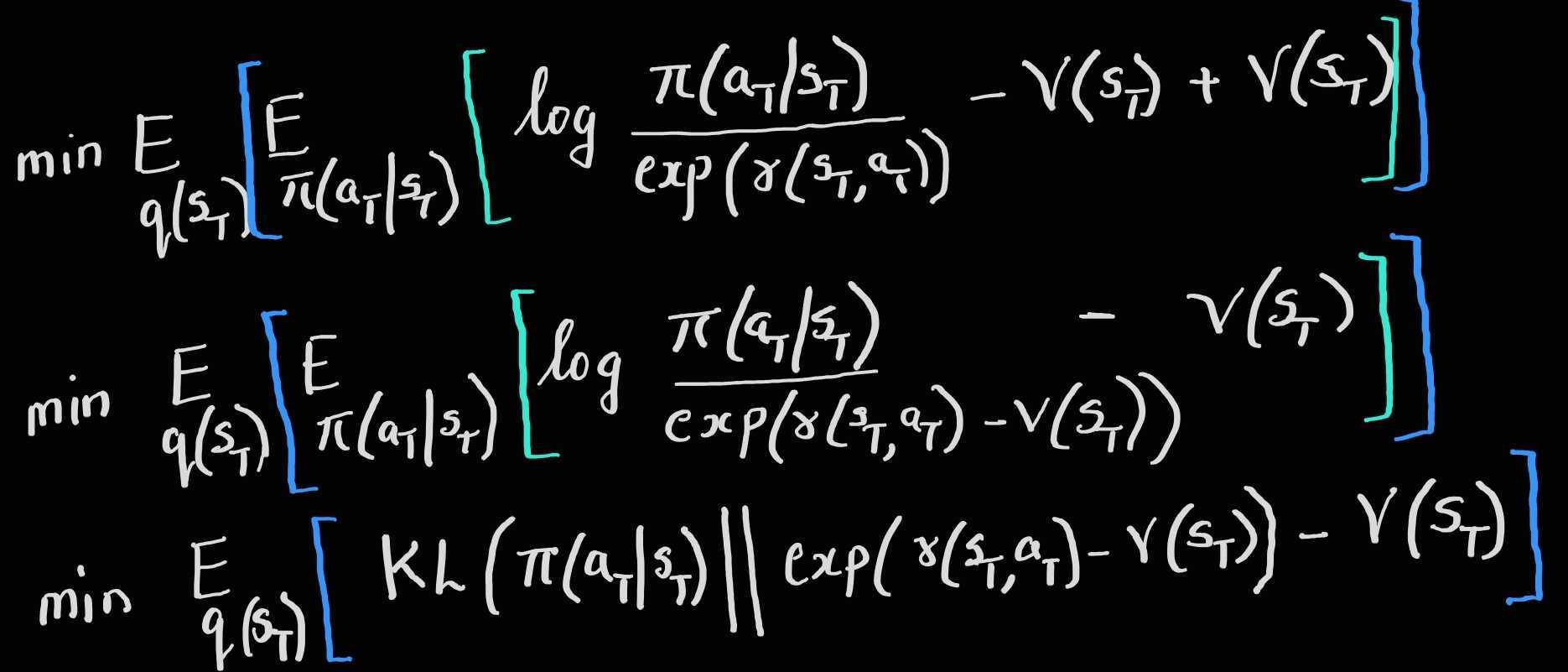
At the last time step T

However, note that here we consider a general scenario where the reward can take any real value, $-\infty < r(s,a) < \infty$ , as opposed to the earlier restriction to be negative or zero. Thus we need to normalize $\exp(\log(r(s_T,a_T)))$, using the normalizing constant $V(s_T)=\int_{\mathbb{A}}\exp(r(s_T,a_T)) da_T$.
Thus we do a little bit more algebraic manipulation to include this normalization constant as follows:

The optimal policy that minimizes this objective is given as :
\[\begin{aligned} \color{green}\pi^*\left(\mathbf{a}_{T} \mid \mathbf{s}_{T}\right)&=\exp \left(r\left(\mathbf{s}_{T}, \mathbf{a}_{T}\right)-V\left(\mathbf{s}_{T}\right)\right)\\ \color{green}V\left(\mathbf{s}_{T}\right)&=\log \int_{\mathcal{A}} \exp \left(r\left(\mathbf{s}_{T}, \mathbf{a}_{T}\right)\right) d \mathbf{a}_{T}\\ &\approx\underset{\mathbb{A}}{softmax}\left(r\left(\mathbf{s}_{T}, \mathbf{a}_{T}\right)\right) \end{aligned}\]At any time step t,

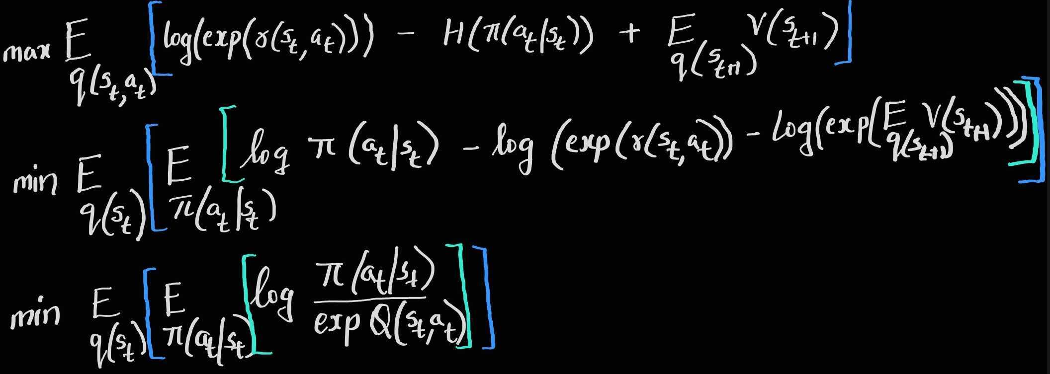
The optimal policy that minimizes this objective at any time step t is given as :
\[\begin{aligned} \color{green}\pi^*\left(\mathbf{a}_{T} \mid \mathbf{s}_{T}\right)&=\exp \left(Q\left(\mathbf{s}_{T}, \mathbf{a}_{T}\right)-V\left(\mathbf{s}_{T}\right)\right)\\ \color{green}Q\left(\mathbf{s}_{t}, \mathbf{a}_{t}\right)&=r\left(\mathbf{s}_{t}, \mathbf{a}_{t}\right)+E_{\mathbf{s}_{t+1} \sim p\left(\mathbf{s}_{t+1} \mid \mathbf{s}_{t}, \mathbf{a}_{t}\right)}\left[V\left(\mathbf{s}_{t+1}\right)\right]\\ \color{green}V\left(\mathbf{s}_{T}\right)&=\log \int_{\mathcal{A}} \exp \left(Q\left(\mathbf{s}_{T}, \mathbf{a}_{T}\right)\right) d \mathbf{a}_{T}\\ &\approx\underset{\mathbb{A}}{softmax}\left(Q\left(\mathbf{s}_{T}, \mathbf{a}_{T}\right)\right) \end{aligned}\]This means that, if we fix the dynamics and initial state distribution, and only allow the policy to change, we recover a Bellman backup operator that uses the expected value of the next state, rather than the optimistic estimate we saw in part 2 of the blog series. Thus we avoid the risk seeking behaviour / optimistic bellman backups via the control as inference framework.
We will discuss how this framework is used practically in modern Deep RL alogorithms in the next part of this blog series.