Control As Inference In PGMs (Part 2) - Policy Search Via Exact Inference

Viewing policy search as an exact inference procedure in a graphical model

In the 1st part of the blog series on control as inference, we discussed why this paradigm is interesting. In the second part of the blog, we will discuss how we can treat policy search as exact inference in this graphical model via variable elimination.

We will see that the subroutines in the policy search procedure in this graphical model result in “soft” variations of bellman update equations, where the hard max in operation is replaced by a softmax.

Log Sum Exp Trick

A useful “trick” to remember before we jump into control as inference procedure is “Log Sum Exp” trick. The LogSumExp (LSE) (also called RealSoftMax or multivariable softplus) function is defined as the logarithm of the sum of the exponentials of the arguments:

\[\operatorname{LSE}\left(x_{1}, \ldots, x_{n}\right)=\log \left(\exp \left(x_{1}\right)+\cdots+\exp \left(x_{n}\right)\right)\]

The LSE function is a smooth maximum – a smooth approximation to the maximum function, mainly used by machine learning algorithms. In the following inference procedure, we will replace LSE with max/softmax to derive a soft version of classical RL.

Exact Inference By Recursive Computation Of Backward Messages

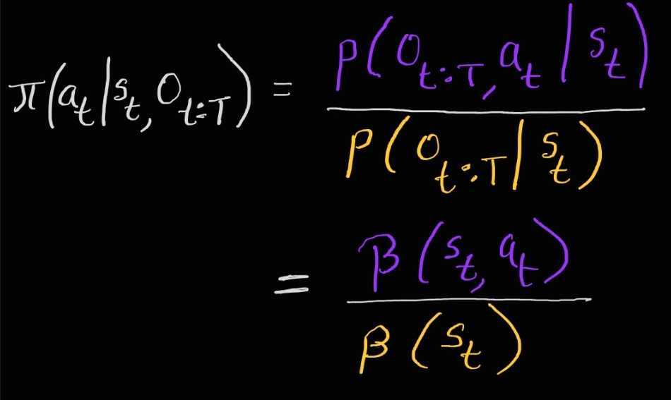
At any time t policy search involves computing the posterior over the action $a_t$, given state $s_t$ and the optimality variables $O_{t:T}$, i.e.

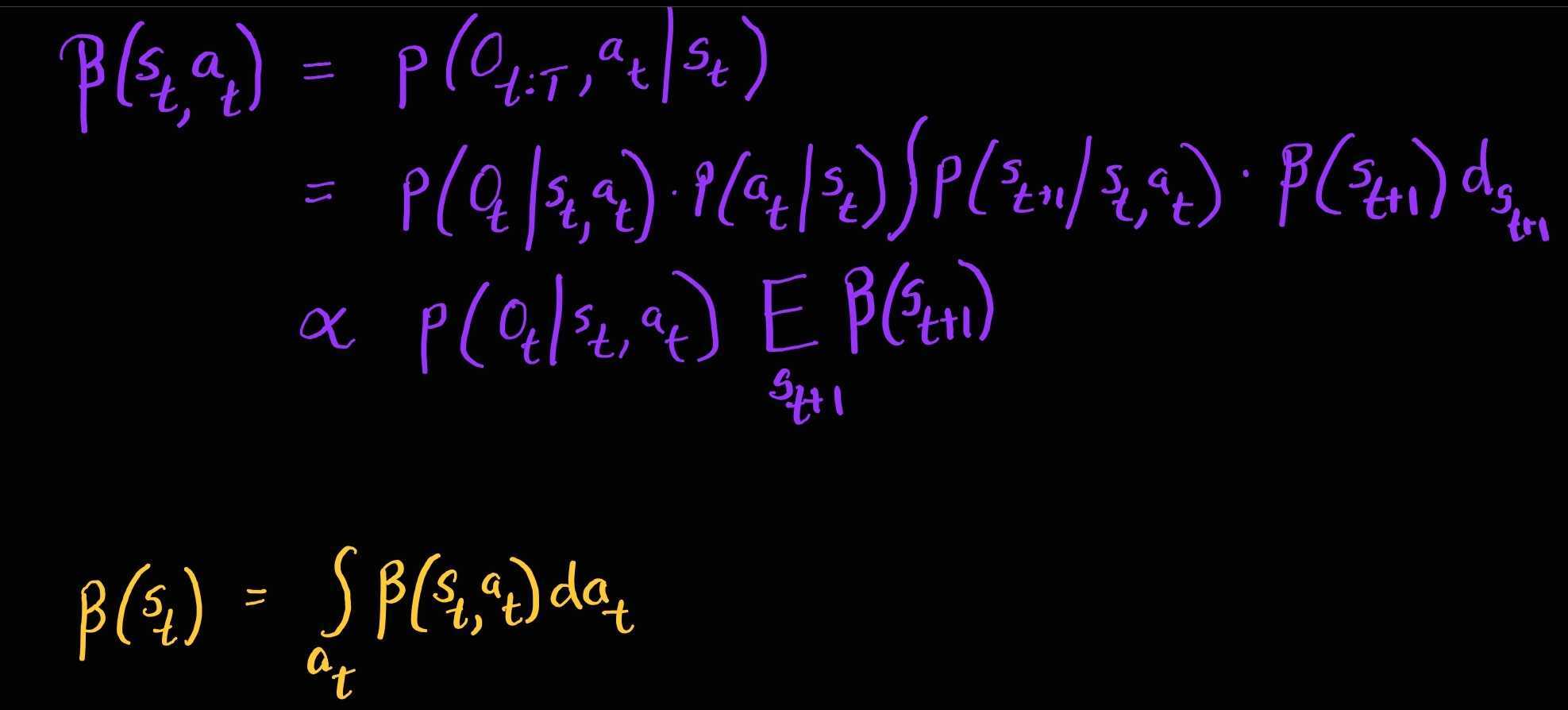
Thus policy search involves computing two backward messages \(\color{orange} \beta_{t}\left(\mathbf{s}_{t}\right)\) and \(\color{purple} \beta_{t}\left(\mathbf{s}_{t},\mathbf{a}_{t}\right)\). This is computed via backward messages similar to HMM or Kalman Smoothers as follows:

At the last time step T:

Note on Action Prior: Here $p(a_t \mid s_t)$ is the action prior. Note that it is not conditioned on $O_{1:T}$ in any way, i.e. it does not denote the probability of an optimal action, but simply the prior probability of actions. The PGM for RL as inference doesn’t actually contain this factor, and we can assume that $ p\left(a_t \mid s_t \right)= \frac{1}{ \mid \mathcal{A} \mid} $ for simplicity. That is, it is a constant corresponding to a uniform distribution over the set of actions.

Thought Exercise:

Levine 2018 assumes a uniform action prior and argues that this assumption does not introduce any loss of generality. One could show that any non-uniform action prior $p(a_t \mid s_t)$ can be incorporated into $p(O_t \mid s_t,a_t):=exp(r_1(s_t,a_t))$ via a modified reward function $r_1(s_t,a_t)$.

At any time step t

Intuition / Relationship To Classical RL

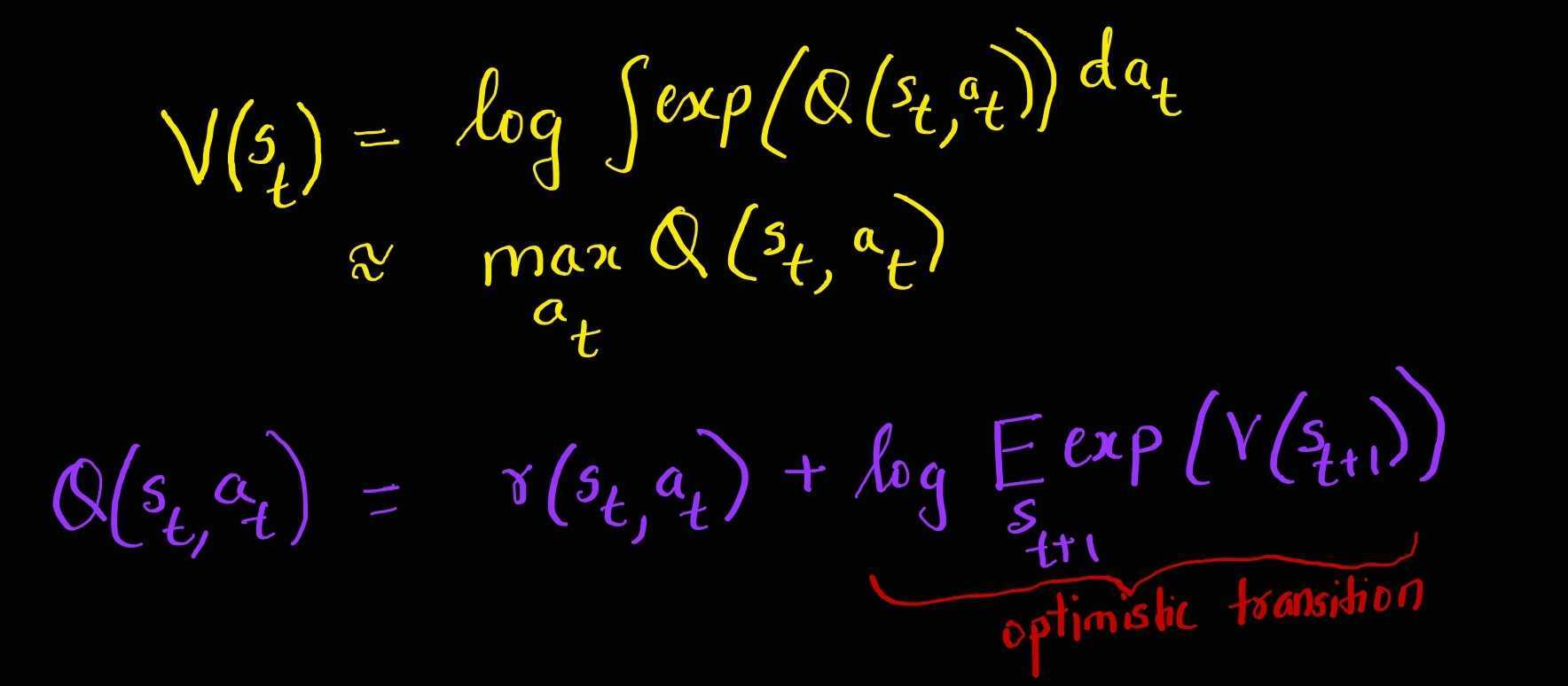
In order to get an intuitive meaning of these messages, we do some algebraic manipulation in the log space to get a form similar to bellman backup. The messages in log space are as follows:

Equation 1: Messages in log space

One can show that if we replace the $\log \beta(s_t,a_t)$ with Q function and $\log \beta(s_t)$ with the value function we can recover an intuitive relationship resembling bellman backup operator in the deterministic case and an optimistic bellman backup in the stochastic case. Let,

\[\begin{aligned} \color{purple} Q\left(\mathbf{s}_{t}, \mathbf{a}_{t} \right) &= \log \beta_{t}\left(\mathbf{s}_{t}, \mathbf{a}_{t} \right) \\ \color{orange}V\left(\mathbf{s}_{t}\right) &= \log \beta_{t}\left(\mathbf{s}_{t} \right) \end{aligned}\]

Equation 2: Relationship between backward messages and Q/Value functions in classical RL.

Using Equations 1 and 2, now the messages in the log space look as follows:

Deterministic Case (Regular Bellman Backup)

In the deterministic case since we only have one possibility for transition dynamics, we obtain a backup equation similar to the regular Bellman backup equation.

\[\color{purple}Q\left(\mathbf{s}_{t}, \mathbf{a}_{t}\right)=\color{black}r\left(\mathbf{s}_{t}, \mathbf{a}_{t}\right)+\color{orange}V\left(\mathbf{s}_{t+1}\right)\]

Stochastic Case (Optimistic Backup)

In the stochastic case we obtain a backup equation that is optimistic as shown below:

\[\color{purple}Q\left(\mathbf{s}_{t}, \mathbf{a}_{t}\right)=\color{black}r\left(\mathbf{s}_{t}, \mathbf{a}_{t}\right)+\log E_{\mathbf{s}_{t+1} \sim p\left(\mathbf{s}_{t+1} \mid \mathbf{s}_{t}, \mathbf{a}_{t}\right)}\left[\exp \left(\color{orange}V\left(\mathbf{s}_{t+1}\color{black}\right)\right)\right]\]

The optimistic update occurs because it is largely determined by the max of the next state value, which creates risk-seeking behaviour.

This issue will be mitigated by variational inference discussed in the next part of this blog series.